Batch mode sorting was added to SQL Server in the 2016 release under compatibility level 130. Most of the time, a batch mode sort will be much faster than the row mode equivalent.
This post is about an important exception to this rule, as recently reported by Erik Darling (video).
No doubt you’ll visit both links before reading on, but to summarize, the issue is that batch mode sorts are very slow when they spill—much slower than an equivalent row mode sort.
This also seems like a good opportunity to write down some sorting details I haven’t really covered before. If you’re not interested in those details and background to the current issue, you can skip down to the section titled, “Erik’s Demo”.
Previous Parallel Batch Mode Sort Issue
One exception to the better performance goal of batch sorts was quicky noticed by the community and addressed in SQL Server 2016 CU1: Although a parallel batch mode sort performs its sorting work using multiple threads, the final sorted output is provided on a single thread.
Providing sorted output across multiple threads requires the upstream operator to be aware of the arrangement so it can account for each row’s position in the global sort order. Since the 2016 release, only the new batch mode Window Aggregate operator has been so equipped.
In parallel plans where the parent of a batch mode sort is parallel and not a Window Aggregate, performance suffers because the parallel parent operator receives its entire input on a single thread.
Microsoft addressed this by disallowing parallel plan shapes where a batch mode sort is not followed by a Window Aggregate or Gather Streams operator. It’s a bit rich to call it a ‘fix’ but that’s the situation we have today, even in SQL Server 2022.
It’s not the issue that causes slow batch mode sort spills, but it is slightly related, so I mention it for historical context and completeness.
Row Mode Sorts
A quick description of row mode sorts for comparison purposes. The implementation is largely the same as originally released with the epic SQL Server 7 release.
The most notable change since then has probably been the addition of resumable sorts (patent) for resumable online index builds, implemented as a complete spill to persistent storage along with the metadata needed to restart the sort at a later time, perhaps at a different degree of parallelism (DOP).
At a high level, a row mode sort reads a row at a time from its child operator and copies the row data into reserved sort memory. This continues until the source of rows is exhausted or the sort runs out of memory grant.
If the input data fits in the granted memory, the data is sorted using an internal merge sort algorithm. The sort then transitions to output mode and provides sorted output a row at a time to its parent operator, on demand.
As a reminder, here is the oft-cited (public domain) merge sort diagram:

People have asked in the past for a little more detail about SQL Server’s internal merge sort, so the rest of this section is about that. It’s just background information really, so you can skip it if you are not one of those people.
Internal merge sort
The internal merge sort is arranged as a bottom-up sort of a linked list, where the items in the list are compactly formatted 8KB pages with the sorting key(s) as index keys.
Page formatting somewhat depends on the input data but is generally similar to a nonclustered index page. However, it is different enough that DBCC PAGE will not decode it in detail. Most often, the page will use the familiar FixedVar format but different arrangements can be used if the data source requires it (for example, wide tables, sparse data, compression).
The usual page offset array of pointers to rows provides a convenient way to reorder rows on a page without physically moving potentially large rows around or coding special handling for LOB and row overflow data. The linked list aspect is provided by the normal previous and next page pointers.
Sorting is initially performed per page using the desired ordering keys. If the keys are long, SQL Server may use a key prefix for an initial check, only testing the full values if the short keys compare equal. Comparison is generally performed by calling out to a function. but can be inlined using optimized code for certain data types as I described in my previous post.
Row mode sorting code is quite spread out in the sqlmin DLL, but the core activities are contained in lmmerge, lmpage, lmnext, and lmAddCurToList. The overall operation is quite similar to the pseudocode listed on Wikipedia, including the depth limit of 32.
I like to think the lm prefix on the code method names stands for ‘list merge’ but I don’t know if that’s accurate.
Row Mode Spills
If a row mode sort runs out of granted memory, it usually spills to tempdb. The main exception to that rule is for index building sorts, which may try to request additional memory instead of spilling. Top N sorts where N <= 100 also never need to spill because they only ever keep the top N results in memory (more details in a previous post).
Anyway, in the normal course of events, a row mode sort switches to an external merge sort when memory runs out.
External merge
The data currently in memory is sorted and then written out to a tempdb workfile as a sorted run. Memory is then freed up for more input records, which are then sorted and written out to a new sorted run. This process repeats until the input is exhausted.
At this point, we have some number of sorted runs in tempdb storage. To produce the final sorted output, we need to merge these runs. Depending on the memory grant, this might need more than one pass over the data. Most often, a single pass is sufficient.
It is not efficient to read one row from each run workfile at a time, so we need one or more memory buffers per run. We read a chunk of data (64KB) from each run into memory buffers and perform a k-way merge from there.
Since each run requires one or more buffers for optimal performance, there is a maximum number of runs we can merge at the same time. This is known as the fan-in. When the number of runs exceeds the fan-in, a multi-pass merge is performed.
For example, say we end up with 100 sorted runs and our maximum fan-in is 20. The first pass performs five separate 20-way merges resulting in five new sort runs. The second pass then performs a five-way merge of these larger runs to start streaming the final sorted output.
Larger inputs and smaller memory grants may require more merge passes. The general idea is that each merge pass reduces the number of sorted runs (and increases their length) until a final merge is possible using the granted memory mostly for input and output buffers.
Optimising comparisons
The k-way merge does not compare the first item of every run each time it is asked for the next row in sorted order. That would be very inefficient with a large number of runs.
Instead, a tournament tree of losers is maintained, which reduces the average number of comparisons to log k.
Dynamic transition
An interesting aspect of the SQL Server implementation is that a sort that is just one row too large to fit in granted memory will spill the entire memory contents to a tempdb workfile. The single row will be written to a second run, then an external merge performed on those two runs to produce sorted output.
It is possible in theory to write just enough data to a workfile to enable the final row to be read into memory, then merge memory with the one row from the workfile. SQL Server doesn’t do this today though I must admit I thought it did in the past. Perhaps managing rows of different lengths is too difficult, or the extra work just doesn’t pay off often enough to justify the additional complexity. Perhaps there was some edge case bug. Perhaps I imagined the whole thing.
Memory use
Row mode sorts are somewhat pessimistic. SQL Server reserves a relatively small portion of the granted memory for structures (e.g. big output buffers, or ‘bobs’) needed to manage and optimize spill throughput. It does this even if the sort doesn’t spill. This memory is not available for direct sorting.
Older versions of SQL Server did not account for this overhead correctly when computing estimates and grants. Documented trace flag 7470 was provided to address this.
Currently supported SQL Server versions have the new behaviour enabled by default, though TF 7470 is still checked and has an effect on the calculations. It is not clear under which circumstances it might be needed these days. Something to research another time.
Row mode sort parallelism
SQL Server runs a row mode sort in parallel by creating DOP serial sorts and splitting the memory grant equally between them. Each instance of the sort receives some of input rows as determined by previous operators in the execution plan.
In many cases, rows are assigned to threads by a parallel scan or seek. Other times, an exchange (Repartition Streams) may be necessary to ensure the parallel operators return correct results for the query as a whole.
In any event, skew between threads can result in some instances of the sort spilling, while others have more memory reserved for their use than they ultimately can make use of.
Any synchronization necessary between parallel tasks is performed at exchanges, resulting in the familiar CX* family of waits.
Batch Mode Sorting
The batch mode sort implementation is very different, which is not surprising given the time that elapsed between SQL Server 7 and SQL Server 2016.
Don’t misunderstand me—the row mode implementation is still very decent, but it was written at a time when external storage was slow and largely magnetic, with long disk track seek times and very much better sequential I/O performance than random.
CPUs were also very different back then. Understandably, most of the design effort went into optimising external merge sort and maximising I/O performance.
Internal merge sort was a natural and convenient choice for the in-memory sorting, but it was considered a relatively unimportant aspect. Few people were paying serious attention to CPU, cache, or main memory performance considerations back then.
Modern considerations
Batch mode sorts place the emphasis very firmly on modern considerations like SIMD, CPU cache locality, scalability with a large number of cores, and main memory bandwidth. It even has an eye on cutting-edge developments like GPU use for sorting.
Like most modern sorting implementations, batch mode sorts use a hybrid sort known as introspective sort or introsort. This uses quicksort most often, insertion sort for very small inputs, and switches from quicksort to heapsort when too much quicksort partitioning is found to be necessary at runtime.
Why batch sorting is faster
Quicksort is usually preferred over internal merge sort these days because although it performs more comparisons on average, quicksort has much better CPU cache locality (instructions and data are much more likely to be in near-CPU caches). This is very much the determining performance consideration these days.
SQL Server has optimized implementations for heapsort, quicksort, and insertion sort for all the main built-in data types. The interested reader with a debugger is directed to sqlmin DLL entries for CBpsortLocalSort::InsertionSort, CBpsortLocalSort::QuickSort, CBpsortHeap::* and the hundreds of anonymous lambda functions.
Batch mode sorts are faster than row mode sorts (when all goes well) for many reasons. Receiving data in batches of up to 900 rows is good for CPU cache locality both for data and code instructions. Modern code tends to perform better on modern hardware than legacy code, as you’d expect.
Most of the improvements come from ensuring cores have useful work to do as often as possible, with minimal waits for (relatively) very slow main memory. Even single-threaded batch mode sorts benefit from CPU-optimized code and cache awareness.
Parallelism
Batch sorts don’t use exchange operators like Repartition Streams for parallel synchronization, but this doesn’t mean they magically don’t need to coordinate work among threads. Instead, batch operators use synchronization points (‘sync points’) using OS synchronization objects.
The generic BPSORT wait type is associated with waiting at a sync point. The public code contains string descriptions for the sync point waits classified as BPSORT, but the strings are not currently exposed by any extended events.
The BPSORT sync point strings are:
SortStartDataAccumulatedInMemSortStartLocalSortDoneMergeTaskPreparedMergeTaskExecutedRemainingStreamCopiedInMemSortEndSpillEndSpillDataLoadPreparedStepN(N = 1-3)SpillSortPreparedMergeRoundStartMergeStreamLoadedMergeStreamPreparedFromSpillLeftoverRowsMovedMergeRoundEndMergeEndOutputScanInitializedSpillDataFinalLoadPreparedStepN(N = 1-5)OutputDataLoaded
Batch mode sorts were written with parallelism in mind. When serial batch mode processing came along later, a special implementation was not written for this case. A serial batch sort still encounters sync points, but never finds anything to wait for. It is truly a parallel batch mode sort running at DOP 1.
Batch sorts were also designed to share granted memory among threads and acquire extra memory as needed. The latter behaviour is not fully enabled at present without a trace flag. In any case, a batch sort will respect a hard limit on memory use like a MAX_GRANT_PERCENT hint or Resource Governor setting.
Merging sorted data
Although batch mode sorts usually use quicksort for in-memory sorting, it still needs to merge sorted data sets at times. A parallel sort at DOP 8 might sort in-memory data into eight locally sorted data sets, but these still need to be merged to produce the final ordering. Equally, any data spilled to workfile runs is only sorted within the run and needs to be merged with other runs to provide final results.
It is surprisingly involved to find a good way to distribute the work of merging sorted data sets among threads in a way that provides load balancing, maximizes throughput, and minimizes synchronization.
The SQL Server team chose a technique called Merge Path, which is described by its authors as “a synchronization-free, cache-efficient merging algorithm”. I’m not going to attempt to summarize it further, but anyone interested can read the original paper (PDF).
Spill level
Originally, batch mode sorts didn’t report spill details at all. They do now, but always report a spill level of 8. This number is arbitrary and does not correspond to the spill level reported by a row mode sort or reflect spill level as we usually understand it.
Microsoft explain this by saying batch mode sorts use a different algorithm where spill level doesn’t really apply in the same way. More on that shortly.
Erik’s Demo
Erik’s query sorts a data set but returns no rows, so timing isn’t affected by client display times:
SELECT
    CN.*
FROM
(
    SELECT
        C.*,
        n = ROW_NUMBER() OVER (
            PARTITION BY C.UserId
            ORDER BY C.Score DESC)
    FROM dbo.Comments AS C
) AS CN
WHERE
    CN.n = 0
OPTION
(
    RECOMPILE,
    MAX_GRANT_PERCENT = 1
);
I’m using the Stack Overflow 2010 database and SQL Server 2022 CU9 with 16GB max server memory.
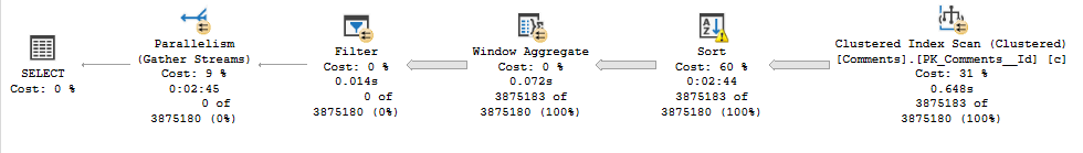
I found the batch mode sort ran for 2 min 45 s at DOP 12:
The row mode sort took only 2.2s:

With a MAXDOP 1 hint, the row mode sort ran for 5,353 ms and the batch mode sort ran for 55,821 ms. That’s still 10x slower, but better than the 75x slower in the parallel case.
Why so slow?
The batch mode sort writes and reads much more tempdb data than the row mode equivalent. It also writes and reads more slowly, if you have reasonably fast local storage.
The following Performance Monitor trace shows the I/O patterns for a row mode sort (left) and batch mode sort (right) running Erik’s spill demo at DOP 1:

The blue line represents bytes written per second and the green line is bytes read per second. The y-axis scale goes up to 1000MB/sec. Red is CPU usage.
Parallelism
I chose to run at DOP 1 because it makes the peaks and pattern easier to see. At DOP 12, the row mode sort is a very sharp peak.
In contrast, the batch mode sort at DOP 12 quickly drops to a miserable level of throughput:

The screenshot shows only the first 60 seconds or so but the drop down to 10-20MB/sec transfer rates is very clear. I haven’t shown the row mode sort on that visual.
Ok, the batch mode sort reads and writes more data, and does so less quickly, especially when parallelism is employed. But why?
Spilling and Merging
The row mode sort is fast and efficient because it performs a single k-way merge of multiple sorted runs.
In one test at DOP 1, the row mode sort wrote k=68 sorted runs to tempdb and merged them all in a single pass.
As an aside, SQL Server was prepared to merge up to 128 runs in a single pass with a 1% maximum memory grant for the default pool with max server memory of 16GB. Beyond that, multiple passes would have been needed. The run thresholds were hardcoded a long time ago when common memory sizes were much smaller. Modern systems could usefully perform larger merges, but no one has updated SQL Server to account for that possibility.
Anyway, the first difference with the batch mode sort is that it initially writes 79 runs to tempdb in 178 workfiles. Why double the number of files? One file is used for regular in-batch data, the other is used for ‘deep data’.
Deep data is used for any column value that does not fit in 64 bits (roughly speaking—see my article Batch Mode Normalization and Performance for details of exactly which data types and values can be stored in-batch).
This is analogous to a row mode sort writing row-overflow and LOB data separately, though deep data is much more common.
This first difference is interesting but quite unimportant as it turns out. The determining factor is what happens after the initial runs are written to tempdb.
Remember when I said batch mode sorts always report a spill level of 8, and Microsoft say this is because batch mode uses a different algorithm?
The different algorithm
Briefly, a detailed analysis of the batchmode_sort_spill_file extended event shows that batch mode sorts use an iterative binary merge for the spilled data. I won’t bore you with the thousand-or-so spreadsheet data entries and cross-references needed to come to that conclusion.
Data from the first memory spill is merged with data from the second memory spill and written to a new set of workfiles. This repeats for the third and fourth memory spills, and so on.
When the initial memory spills are exhausted, SQL Server continues with the result of the first merge, then the second merge, and so on until we eventually end up with a fully sorted set of data in tempdb, spread across a number of final workfiles.
I provide that as a summary of the process to assist in understanding. There are more important details, which I will cover next for the interested reader.
Details
As soon as SQL Server realises it cannot complete the batch mode sort within granted memory, it requests small ad-hoc memory grants for the initial structures needed to support spilling. This optimistic approach is in contrast to the row mode strategy of creating the necessary structures up front from granted memory.
SQL Server then starts writing workfiles for batch and deep data to tempdb as described previously. Each time memory fills with data it is sorted then gradually written to tempdb in multiple workfiles, consisting of a row data workfile and an associated deep data workfile if needed. The deep data is associated with a dictionary and has an observed maximum size around 12.5MB.
Each write has a start_row_id to indicate its position within the local sort order. The row id resets to zero each time memory is cleared before reading more input data. For example, the first memory spill might result in four row data workfiles (each with an associated deep data workfile):
- File 1, start row id 0
- File 2, start row id 49,104
- File 3, start row id 78,207
- File 4, start row id 117,463
The batch mode sort then transitions to spill_stage 4 (parallel external merge). This processes a pair of spilled workfile sets at a time, merging the two sets using the Merge Path algorithm to distribute work among parallel threads.
Note this merging does not involve just four (or eight if you count deep data) workfiles. It is the first two main memory spills that are merged, regardless of the number of workfiles they were written to.
The result of the merge is a new set of workfiles with updated start_row_id values reflecting the merged data order.
This binary merge process continues as mentioned in the preceding summary until we eventually end up with a single set of workfiles in sorted order running from start_row_id zero to the number of rows in the complete data set.
The problem
An iterative binary merge is a fine algorithm for an in-memory merge sort. It is a terrible choice for merging spilled data because the result of each mini merge has to be written to persistent storage, potentially many times.
Each data item may be written and read multiple times but how many times this happens to a particular item depends on its position in the initial data stream and its final sort order. Since different items may participate in a different number of merge steps, it doesn’t make sense to report a single spill level for the operation as a whole.
In principle, SQL Server could record an average number of merge steps, but this would usually (and meaningfully) be a fractional number. People might find a spill level of 2.6 confusing. Besides that, spill level is currently defined in showplan as an integer.
Anyway, the use of binary merge explains why the Performance Monitor trace shows so much more data being written and read with the batch mode sort.
The situation is made worse when parallelism is involved because the (deliberately) limited amount of memory is further split into DOP partitions. Each spilled workfile ends up being smaller than is ideal for I/O purposes.
In addition, there are DOP more merging subtasks. In short, everything gets worse.
Conclusion
A great deal of care and attention has gone into making batch mode sorts fast when the input is large and sufficient of memory is available. Much effort has been expended to take advantage of modern CPU & memory architecture characteristics, while making full and efficient use of the larger number of cores typically available.
It is hard to believe then, that the iterative binary merge for spilled workfiles is deliberate. It’s just such an obviously inappropriate choice that it must be the result of an oversight, whether that is in the functional specification or coding implementation.
Perhaps it performs acceptably well when a very large data set is spilled, and the low memory scenario is an untested edge case? In any event, it is not hard to find instances of terribly slow batch mode sort spills in real environments once you start looking for them. Clearly, a fix is needed.
Avoiding a traditional k-way merge is somewhat understandable because the required tournament tree of losers has poor cache locality. That aspect fits with what appears to be the overall design philosophy here.
None of that makes up for the awful performance delivered by the current implementation under limited memory conditions. We will have to see how Microsoft respond. At the time of writing, the only comment on the feedback item is:
Thank you for providing the plans and repro details. We are able to reproduce the behavior and are discussing next steps.
Appreciate the effort that went into this article, and how well it is written. I hope I never see the slowdown in the flesh, but at least I'll have a clue what it is if I do see it.
ReplyDeleteGreat deep dive on this, thanks.
ReplyDelete